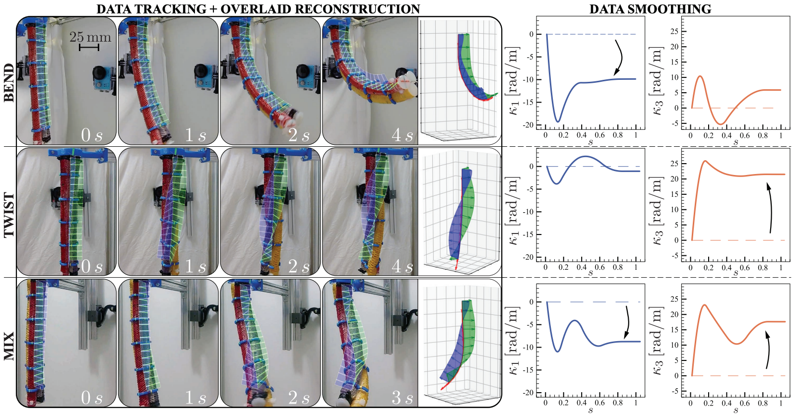
Take a flexible tube and twist one end. Its center line can remain almost unchanged, even though the material has undergone a substantial deformation. Now bend it while twisting, or let neighboring cross-sections slide sideways relative to one another. A picture of the tube's outline becomes even less informative about what is happening inside its motion.
This is a measurement problem for soft robotics and biomechanics: how can we recover the way a slender body deforms, along its entire length, from a few camera observations?
In our paper, A physics-informed, vision-based method to reconstruct all deformation modes in slender bodies, Seung Hyun Kim, Chia-Hsien Shih, Naveen Kumar Uppalapati, Udit Halder, Girish Krishnan, Prashant G. Mehta, Mattia Gazzola, and I combine multi-camera tracking with Cosserat rod mechanics. The result is an estimate of both the body's three-dimensional pose and its six strain fields, including twist and shear.
The cameras supply discrete observations. Mechanics helps connect them into a continuous body.
Reconstruction in action
A center line is only part of the shape
A Cosserat rod represents a slender body with two ingredients at every location along its length: a position $\mathbf r(s)$ and an orientation $Q(s)$. Here, $s$ labels position along the reference length of the arm. The columns of $Q$ are three perpendicular unit vectors, called directors, attached to each cross-section.
Two directors span the cross-section; the third is perpendicular to it. That third director need not align with the center-line tangent. Their misalignment is precisely what allows the model to describe shear.
The changes in position and orientation are governed by six components:
| Deformation | Components | What changes locally |
|---|---|---|
| Bending | $\kappa_1,\kappa_2$ | Cross-sections rotate about their two transverse axes |
| Twisting | $\kappa_3$ | Cross-sections rotate about their own normal axis |
| Shearing | $\nu_1,\nu_2$ | Neighboring cross-sections shift sideways relative to the local frame |
| Stretching | $\nu_3$ | Separation changes along the cross-section normal; the undeformed value is 1 for a straight, unstretched rod |
With $Q$ mapping local coordinates into the laboratory frame, the rod's kinematics can be written as
$$ \frac{d\mathbf r}{ds}=Q\boldsymbol\nu, \qquad \frac{dQ}{ds}=Q[\boldsymbol\kappa]_\times. $$
The notation $[\boldsymbol\kappa]_\times$ denotes the matrix that takes a cross product with $\boldsymbol\kappa$. Given these strain fields and a base pose, we can integrate the equations to reconstruct the rod.
The inverse problem goes the other way: use measured positions and orientations to infer the strains. Tracking cross-section markers makes orientation observable, which is essential for distinguishing a straight, twisted arm from a straight, untwisted one.
From five cameras to discrete poses
Our laboratory setup surrounds the arm with five action cameras recording at 60 frames per second and 1080p. The cameras are arranged so that each tracked marker point is visible in at least two views over the intended motions.
Before tracking the arm, we calibrate the cameras throughout a $40\times30\times40$ cm workspace. Colored flags hang along weighted nylon wires, and moving this grid through the volume provides more than 1,000 reference points. The reported calibration errors are 1.4 mm on average and 2.6 mm at maximum.
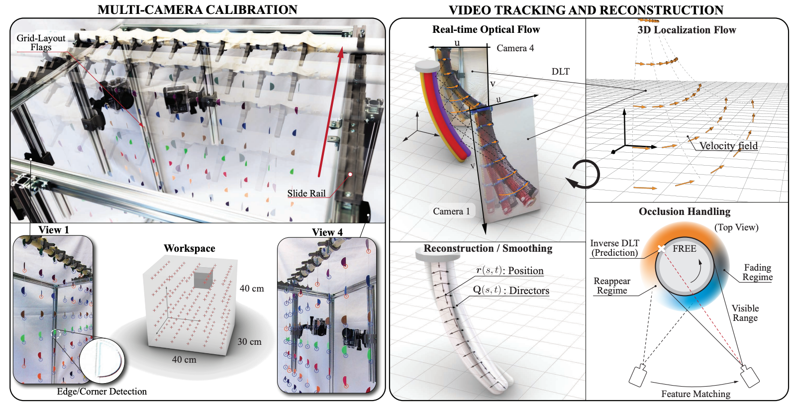
Calibrate, track, reconstruct. Multiple views provide discrete three-dimensional marker positions and cross-section orientations. The rightmost panel illustrates how other camera views help recover a marker when it reappears. Figure 2 from the preprint.
After an initial manual selection, Lucas–Kanade optical flow follows marker points through successive images. Direct Linear Transformation (DLT) combines the calibrated views to estimate their three-dimensional coordinates. The cross-section markers then supply discrete position-and-orientation measurements along the arm.
Multiple views also help with occlusion. When a point disappears from one camera but remains visible to others, its reconstructed position predicts where to look for it when it reappears. This depends on sufficient camera coverage; the method cannot observe a marker hidden from every view.
Let mechanics fill the gaps
Directly differentiating noisy pose measurements can produce unreliable strains. Fitting independent rod segments between successive markers also creates a problem: the segments may meet in position and orientation while their strains jump at the boundaries.
We instead optimize a single rod over its full length. Three terms guide the estimate: an elastic energy, a penalty on rapid spatial changes in strain, and a mismatch cost for the measured poses.
Collect the six strains into $\varepsilon=(\boldsymbol\kappa,\boldsymbol\nu)$, and let $\varepsilon^\circ$ be their intrinsic, stress-free values. Using the paper's quadratic elastic model, the objective is
$$ \begin{aligned} J={}&\frac12\int_0^L (\varepsilon-\varepsilon^\circ)^T R(s) (\varepsilon-\varepsilon^\circ)\,ds\\ &+\frac{\chi_u}{2}\int_0^L \left\|\frac{d\varepsilon}{ds}\right\|^2\,ds\\ &+\sum_j\left[ \frac{\chi_r}{2}\|\mathbf r(s_j)-\mathbf r_j\|^2 +\frac{\chi_Q}{2}\|Q(s_j)-Q_j\|_F^2 \right]. \end{aligned} $$
Here, $R(s)$ is the rigidity matrix, $(\mathbf r_j,Q_j)$ are measured poses, and the positive weights $\chi_u,\chi_r,\chi_Q$ balance smoothness and data agreement. The Frobenius norm $\lVert\cdot\rVert_F$ measures the orientation-matrix mismatch.
The elastic term gives different deformations a mechanical cost. The strain-gradient term discourages abrupt variation. The measurement term keeps the reconstruction close to the observations without forcing it to pass exactly through noisy data. Together, these terms express what physics-informed reconstruction means in this work: rod kinematics constrain the geometry, and elasticity supplies a mechanical prior.
The key optimization choice is to treat the spatial derivative of strain, $u(s)=d\varepsilon/ds$, as the control variable. Integrating it produces continuous strain fields. With the base pose and base strain specified, the solver repeatedly:
- Integrates strain and pose forward from base to tip.
- Propagates sensitivity information backward, accounting for the measurement errors at each marker.
- Updates $u(s)$ to reduce the objective.
This is optimal control along the arm's spatial coordinate. The pose costates, which carry sensitivity information backward, can be expressed as internal force and moment. The calculation reconstructs an observed configuration; it does not require prescribing the robot's actuator commands or solving a full time-dependent motion model.
Testing what can be recovered
We first generate synthetic rods from known, smoothly varying strain functions. This gives an exact reference for all six strain components, something much harder to obtain on hardware.
For the tested synthetic curves, the reported relative reconstruction errors fall to roughly 1% with five sampled poses and remain around 5% with two. These are results for the chosen smooth strain profiles, rather than a general sampling rule for every possible soft-body shape.
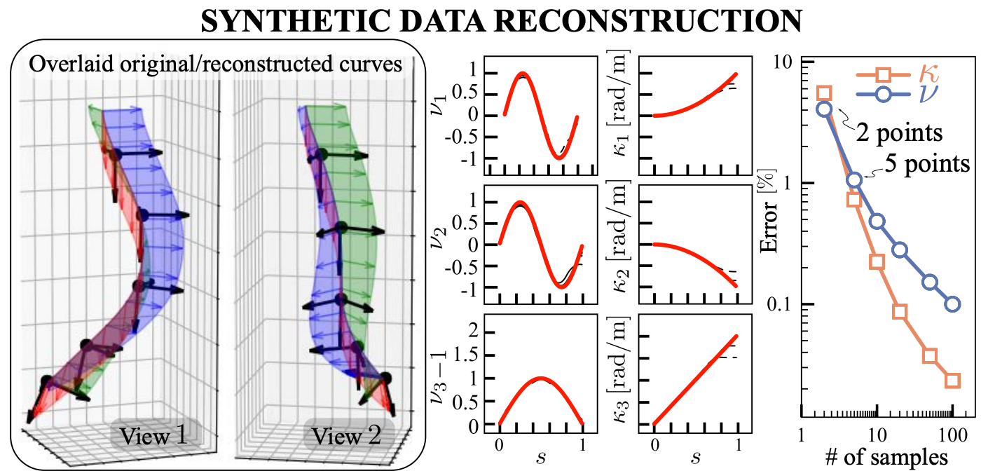
Checking against known strains. Synthetic data makes it possible to compare the recovered strain fields with their generating functions. The right-hand plot varies the number of sampled poses. Figure 3 from the preprint.
For the first hardware experiment, we use an 18 cm pneumatic BR² arm made from three parallel fiber-reinforced elastomeric actuators: one designed to bend and two to twist in opposite directions. Five cross-section markers provide the observations.
The opening figure shows separate bending, twisting, and combined actuation. The recovered strain profiles identify the dominant deformation in each case. They also reveal smaller accompanying deformations caused by mechanical coupling, fabrication effects, and gravity.
To measure position accuracy independently, the published paper compares reconstruction with electromagnetic sensors at the arm's midsection, three-quarter position, and last-marker tip. Each actuation experiment is repeated eight times. Table I reports:
| Actuation condition | Median position error | Maximum position error |
|---|---|---|
| Maximum bending | 4.15 mm | 5.43 mm |
| Maximum twisting | 2.96 mm | 4.03 mm |
| Both | 4.13 mm | 5.13 mm |
These measurements assess the complete pipeline, including calibration and reconstruction. The median errors are about 3–4 mm on an arm with a 15.9 mm diameter. Although the abstract summarizes accuracy as below 5 mm, the table records some larger errors. These are position errors, not independent measurements of the accuracy of every strain component.
Recovering coupled deformations
The more demanding demonstrations use a two-section BR² arm and a cable-driven arm. Their different designs help test whether the reconstruction can capture several deformation modes at once.
In the 38 cm BR² arm, one section receives a bending command and the other a twisting command. Eleven cross-section markers support reconstruction of all six strain fields. The expected bending and twisting dominate their respective sections, while smaller coupled strains appear elsewhere.
The 35 cm cable-driven arm uses twelve markers and bends its two sections in different directions. Its softer construction and cable routing let its cross-sectional holders tilt away from perpendicular to the center line. The reconstructed shear captures this visible feature of the deformation.
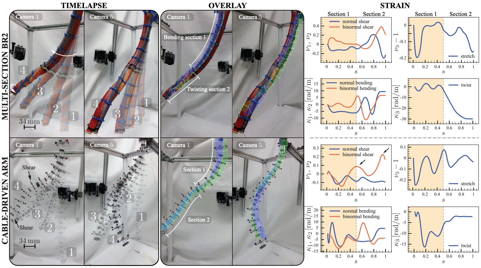
One description for different soft arms. The upper row shows the multi-section BR² arm; the lower row shows the cable-driven arm. Position and orientation overlays connect the camera observations to the recovered strain fields. Figure 5 from the preprint.
We also perturb the cable-driven arm's measured marker positions with uniform noise of up to 5 mm. Reconstructing again changes the strain fields by about 10% on average in the paper's relative $L_2$ measure. This tests sensitivity to added noise by comparing two reconstructions; it is not a comparison with independently known physical strains.
What this makes measurable
The contribution is a way to turn sparse pose observations into a mechanically informed description of a whole slender body. It brings bending, twist, shear, and stretch into the same reconstruction, so an experiment can ask where each deformation occurs and how they interact.
The approach still depends on camera calibration, visible markers, a suitable rod model, specified base conditions, and choices of stiffness and smoothing weights. Fine spatial features between widely spaced markers may be smoothed away. Recording at 60 frames per second also does not establish that the complete reconstruction runs in real time.
The hardware demonstrations support laboratory characterization of soft robots. Applying the method to biological bodies would require suitable tracking and modeling choices. Within that scope, it provides a useful connection between what cameras can observe and what mechanics needs to explain: both where the body is and how its material deforms along its length.
Paper and attribution
This post is based on A physics-informed, vision-based method to reconstruct all deformation modes in slender bodies, by Seung Hyun Kim, Heng-Sheng Chang, Chia-Hsien Shih, Naveen Kumar Uppalapati, Udit Halder, Girish Krishnan, Prashant G. Mehta, and Mattia Gazzola, published in ICRA 2022, pp. 4810–4817.
The experimental error statistics above follow Table I in the published paper. Figures 2–5 are reproduced from the September 17, 2021 arXiv preprint, with surrounding page text and original captions removed and explanatory captions supplied here. The figure assets retain the source's CC BY-NC-SA 4.0 license.
The code repository links to demonstration data and identifies its v0.1 version as the code used to reproduce the paper's results. The BibTeX below cites the published conference paper.
Citation
@inproceedings{kim2022smoothing,
  title = {A physics-informed, vision-based method to reconstruct all deformation modes in slender bodies},
  author = {Kim, Seung Hyun and Chang, Heng-Sheng and Shih, Chia-Hsien and Uppalapati, Naveen Kumar and Halder, Udit and Krishnan, Girish and Mehta, Prashant G. and Gazzola, Mattia},
  booktitle = {2022 International Conference on Robotics and Automation (ICRA)},
  pages = {4810--4817},
  year = {2022},
  doi = {10.1109/ICRA46639.2022.9811909},
  url = {https://doi.org/10.1109/ICRA46639.2022.9811909}
}