A decoder-only transformer predicts the next token by repeatedly updating a sequence of vectors. At each layer, a position can use information from itself and earlier positions. This gives the model a way to revisit earlier observations as it builds a prediction.
Can this familiar layer structure emerge from the mathematics of prediction itself?
In our preprint, Transformer-like Inference from Optimal Control, Aditya Kudre, Prashant G. Mehta, and I approach that question through filtering-control duality. We begin with a probabilistic model of how observations are generated. Minimizing prediction error then becomes an optimal control problem, whose solution defines an inference algorithm called the dual filter.
The resulting algorithm updates a whole sequence of vectors, much like a transformer layer. A controlled experiment also exposes an important difference: when the representation is too small for the assumed hidden-state model, a trained transformer can still make nearly optimal predictions by using the observation history.
Prediction as hidden-state inference
Imagine observing a sequence of symbols produced by a system whose internal state is hidden. To predict the next symbol, we first estimate what that internal state could be.
For a discrete state space with $d$ possible states, the estimate is a probability vector:
$$ \pi_T(x)=\mathbb{P}(X_T=x\mid Z_{1:T}). $$
Here, $X_T$ is the hidden state and $Z_{1:T}$ is the observed sequence. If $C(x,z)$ is the probability that state $x$ emits token $z$, the next-token distribution follows from
$$ \mathbb{P}(Z_{T+1}=z\mid Z_{1:T}) =\sum_{x=1}^{d}\pi_T(x)C(x,z). $$
This is a probabilistic analogue of decoding an internal representation into token probabilities. Each coordinate of $\pi_T$ has a concrete meaning: the probability assigned to one hidden state.
The paper studies two settings. A linear Gaussian model provides a tractable case in which the target is a conditional mean. A discrete-state model brings us closer to token prediction, where the target is a conditional probability distribution. Both lead to a control formulation.
The weights become the controls
The key step is to represent a prediction as a weighted combination of observations. In the nonlinear setting, for a function $f$ of the hidden state, the paper establishes a representation of the form
$$ \pi_T(f)=c_f-\sum_{t=1}^{T}U_{t-1}^{\mathsf T}e(Z_t). $$
The left-hand side is the conditional expectation of $f(X_T)$. Choosing $f$ to indicate a particular state gives that state's posterior probability. On the right, $c_f$ is a deterministic constant, $e$ encodes tokens, and the weights $U_{t-1}$ can depend on the observations preceding $Z_t$. For binary observations, the encoding is simply $e(1)=1$ and $e(0)=-1$.
Although the expression looks like a linear sum, its weights depend on the data, allowing it to represent a nonlinear predictor. Their dependence on past observations also imposes a causal information constraint.
The next step is to choose those weights. For a hidden Markov model (HMM), the duality principle constructs an auxiliary control system and a cost that equals the estimator's mean squared error:
$$ J_T(U;f)=\mathbb{E}\!\left[\bigl(f(X_T)-S_T\bigr)^2\right]. $$
Here, $S_T$ is the estimator associated with the chosen controls. Solving the control problem therefore produces the minimum mean squared error estimate, $\pi_T(f)$. The controls determine how observations contribute to inference; they do not physically steer the system generating the tokens.
There is a useful distinction between the two results. The nonlinear weighted representation applies beyond HMMs, but the paper's explicit nonlinear control formula is derived for the Markovian hidden-state case. The linear Gaussian analysis also handles hidden dynamics with longer memory.
How a layer emerges
For the HMM, the optimal control law depends on the hidden-state probabilities we are trying to compute. Combining that law with the predictor produces a fixed-point equation: the correct probability sequence reproduces itself under the update.
This suggests a layer operation. Start with approximate probability vectors at all $T$ positions, use them to compute controls through the dual equations, and produce a new sequence:
$$ [\rho_1,\ldots,\rho_T] \longmapsto [\rho_1^+,\ldots,\rho_T^+]. $$
Both input and output have shape $d\times T$. Repeating the operation gives a layered inference architecture. The linear Gaussian case has a similar construction using a sequence of auxiliary vectors called momenta, with updates supplied by the optimality equations.
This is the sense in which the architecture is transformer-like: causal sequence-to-sequence updates arise from the inference objective. The derivation does not identify the controls with standard softmax attention, recover every component of a transformer block, or establish a general guarantee that a chosen finite number of iterations reaches the fixed point.
For hidden dynamics with long memory, the linear formulation also offers a computational motivation. It works with a $d\times T$ sequence, whereas a Kalman formulation that explicitly augments the state with the full history must maintain growing covariance matrices. The paper's complexity comparison concerns that history-dependent setting; the number of iterations needed to solve the dual equations remains relevant to practical runtime.
A small experiment with an exact benchmark
To compare control and attention, we use a process that concatenates independently chosen binary patterns. With the paper's main settings, the long pattern has two ones followed by fourteen zeros; the short pattern has one one followed by four zeros. Each new cycle is chosen with equal probability.

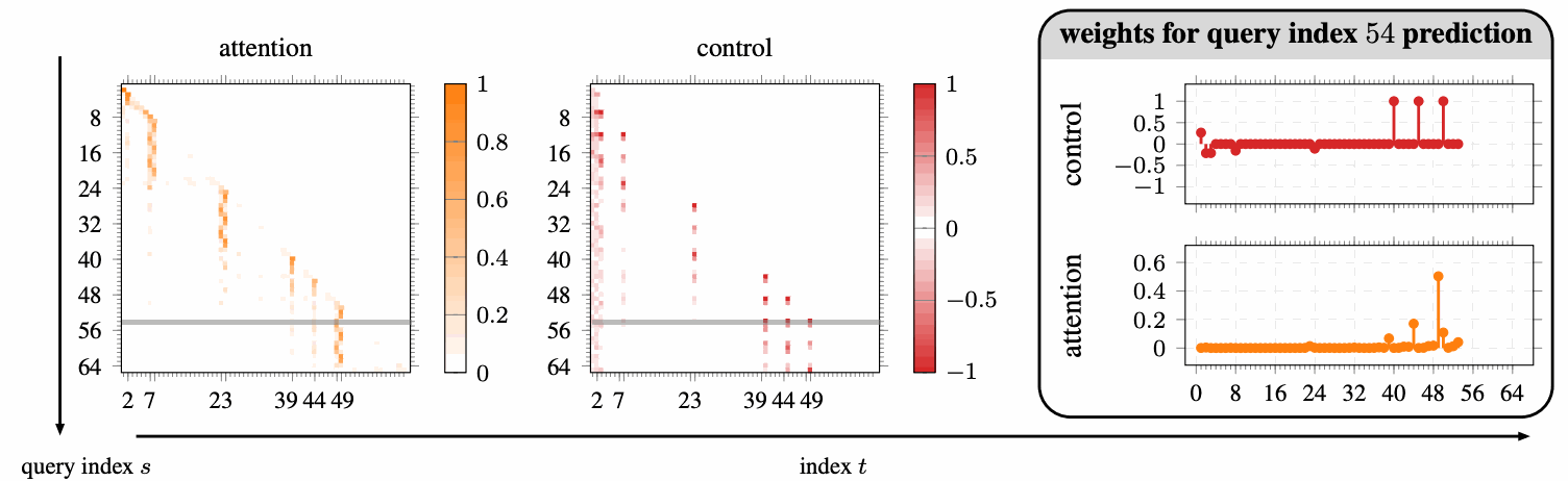
Two cycles, one prediction task. The hidden state tracks progress around the cycles. The locations of the ones help identify that progress. Figure 2 from the paper, with long-cycle length $d=16$ and short-cycle length $q+1=5$.
Because the generating HMM is known, its exact filter provides an optimal next-token prediction benchmark. We train a nanoGPT with one layer and one attention head, using sequences of length $T=64$ and initially an embedding dimension of $16$.
The figure at the top of this post compares its attention weights with dual-filter controls computed from the true HMM parameters. Both emphasize sparse, informative time indices associated with observed ones. The transformer learns this pattern from data, without receiving the HMM parameters.
The resemblance is qualitative. Attention weights are nonnegative and normalized, while the control weights may have either sign. Similar places to look do not imply identical numerical weights or identical computations.
What happens when the representation is too small?
The next experiment holds the true hidden-state dimension at $d=16$ and varies the candidate dimension $\hat d$. For every candidate dimension, the HMM parameters are estimated from data using Baum-Welch; nanoGPT is trained on the same dataset. This differs from the preceding comparison, which used known HMM parameters.
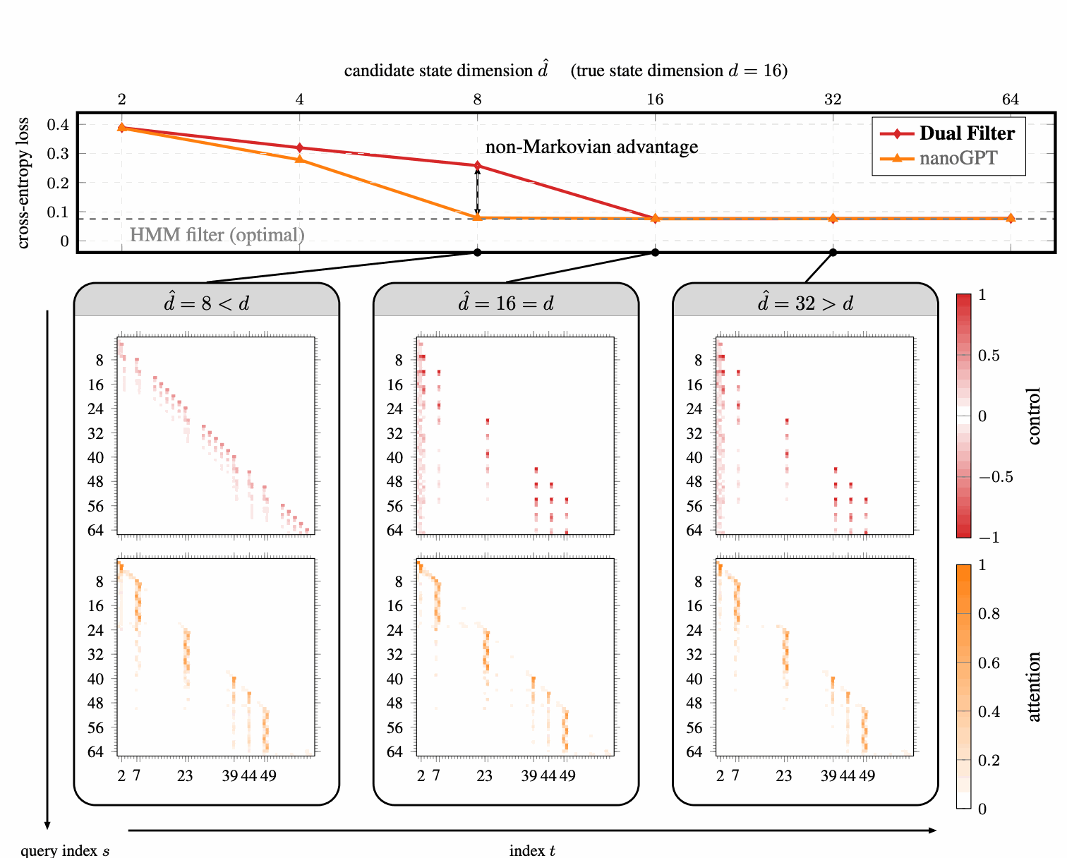
Prediction under a dimension constraint. Lower cross-entropy is better. At $\hat d=8$, nanoGPT stays close to the optimal HMM-filter benchmark while the smaller fitted HMM loses accuracy. The lower panels compare control and attention patterns. Figure 4 from the paper.
When $\hat d\geq16$, both methods achieve near-optimal performance. At $\hat d=8$, the fitted Markovian model loses predictive accuracy, while nanoGPT remains near the benchmark.
We call this a non-Markovian advantage. The smaller HMM must summarize history within an insufficient hidden-state model. Attention can revisit observations across the context, giving the transformer another way to use temporal information.
The underlying data generator is still an HMM. The advantage concerns the restricted representation used for prediction: a smaller embedding dimension does not force a transformer to behave like an HMM with that many states. Nor does matching these dimensions make the two models equal in parameter count or total memory. The experiment identifies a useful gap between these architectures under the tested conditions.
Weight patterns are only part of the story
The appendix tests how the comparison changes when the transition or emission probabilities are perturbed. Each perturbation setting uses a separately trained transformer.
Perturbing transitions changes the optimal controls from a mainly vertical, event-focused pattern to a sparse diagonal pattern that aggregates evidence across past cycles. The transformer's attention remains largely vertical, yet its prediction loss stays near optimal. Perturbing emissions has a smaller effect on the pattern, with weights becoming more diffuse as the perturbation grows.
This makes the interpretation more precise: similar predictive performance can coexist with different weight structures. The experiments do not establish that attention sparsity causes the advantage seen at smaller dimensions.
Where this leads
Filtering-control duality gives a principled route from a prediction objective to a layered inference algorithm. It also gives us interpretable quantities to compare with learned attention: observation weights tied to an explicit probabilistic model and an error criterion.
The present evidence comes from synthetic sequence tasks. Extending the nonlinear control synthesis to hidden dynamics with longer memory, developing a learning framework for the model or the controls, and understanding convergence and computational cost remain important next steps. The undercomplete experiment gives the first of these a concrete target: capture the history dependence that the transformer can exploit.
This connects with the site's earlier posts on Belief Net and transformers and state space models. Here, the organizing connection is between optimal estimation and optimal control: a way to derive an inference architecture from the problem it is meant to solve.
Paper and attribution
This post is based on Transformer-like Inference from Optimal Control, by Aditya Kudre, Heng-Sheng Chang, and Prashant G. Mehta, University of Illinois Urbana-Champaign. The source reviewed here is arXiv:2605.15608v1, submitted May 15, 2026.
Figures 2, 3, and 4 are reproduced as crops from that version. The perturbation study is in Appendix C.2 and Figure 6. The BibTeX citation below refers to the source paper.
Citation
@article{kudre2026transformerlike,
  title = {Transformer-like Inference from Optimal Control},
  author = {Kudre, Aditya and Chang, Heng-Sheng and Mehta, Prashant G.},
  year = {2026},
  eprint = {2605.15608},
  archivePrefix = {arXiv},
  primaryClass = {cs.LG},
  url = {https://arxiv.org/abs/2605.15608}
}