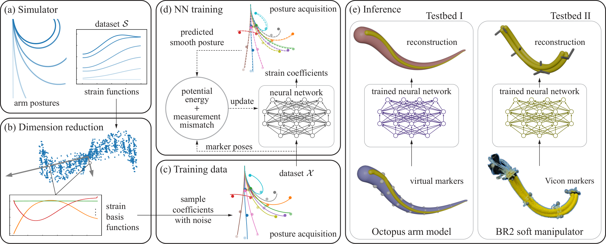
A soft robot needs to know its shape while it moves. A few tracked markers can tell us where selected cross-sections are and how they are oriented, but the arm bends, twists, and stretches continuously between those observations. Recovering that continuous deformation is already difficult. Doing it quickly enough to keep up with motion adds another challenge.
In Seeing How Soft Arms Deform: From Camera Images to Six Strain Fields, I described our earlier method for combining camera measurements with Cosserat rod mechanics. It reconstructs the arm's posture and strain fields by repeatedly solving an optimization problem. The results reveal deformations that an outline alone cannot show, but the calculation can require thousands of iterations for a single frame.
Our follow-up paper, A Neural Network-Based Framework for Fast and Smooth Posture Reconstruction of a Soft Continuum Arm, addresses that bottleneck. Tixian Wang and I, together with our collaborators, develop a neural network that learns the mapping from sparse marker poses to a continuous strain representation. Rod mechanics then turns those strains into the reconstructed arm.
The reported reconstruction benchmark is more than five orders of magnitude faster than the earlier forward-backward algorithm, with comparable normalized objective loss. The central idea is to move the repeated computational effort into training, so a new measurement can be processed with a network evaluation and a spatial integration.
Reconstruction in action
From an optimization problem to a learned map
The earlier approach asks: which smooth deformation best balances mechanical energy, agreement with observations, and the chosen regularization? It integrates the arm's pose from base to tip, propagates a costate backward, and updates the strain description until the optimization converges.
Each measurement set therefore defines a reconstruction problem. Across many frames, these problems have a common structure: the input is a collection of marker poses, and the output is a set of strain fields. We train a network to approximate that input-output relationship.
The input is already a three-dimensional pose estimate. Each marker contributes its position and two perpendicular unit vectors, or directors, describing its orientation. These supply nine numbers per marker; the remaining director follows from orthonormality. The camera or motion-capture system provides these measurements before the network runs.
The output is more subtle. A neural network produces a finite vector, while bending, twist, shear, and stretch vary along the entire arm. We need a way to represent those continuous fields with a small number of numbers.
A small set of patterns describes continuous strain
We begin with simulated motions of the arm and collect the strain profiles that occur along its length. Principal component analysis (PCA) identifies a compact set of spatial patterns that captures the main variations in each strain component.
For strain component $i$, the approximation takes the form
$$ \hat\varepsilon^i(s)=\bar\varepsilon^i_0(s) +\sum_{j=1}^{N_b}\alpha^i_j\bar\varepsilon^i_j(s). $$
Here, $s$ measures location along the reference length, $\bar\varepsilon^i_0$ is the mean strain profile, and the remaining $\bar\varepsilon^i_j$ are basis functions obtained from the simulated data. The coefficients $\alpha^i_j$ tell us how much of each pattern to use. The network predicts those coefficients.
For the simulated octopus arm, four components for each of six strain modes give 24 network outputs. Those 24 values specify strain profiles along the whole arm. This compact representation also limits which deformations the estimator can express: its vocabulary comes from the simulated motions used to construct the basis.
Once the strains are known, we reconstruct position $\mathbf x(s)$ and orientation $Q(s)$ using the Cosserat rod kinematics:
$$ \frac{d\mathbf x}{ds}=Q\boldsymbol\nu, \qquad \frac{dQ}{ds}=Q[\boldsymbol\kappa]_\times. $$
The vector $\boldsymbol\kappa$ contains two bending strains and twist; $\boldsymbol\nu$ contains two shear strains and stretch. The matrix $[\boldsymbol\kappa]_\times$ represents taking a cross product with $\boldsymbol\kappa$. With the base pose specified, integrating these equations connects the predicted local deformations into a complete posture.
Training with mechanics and marker measurements
Collecting dense, accurate strain measurements from a physical soft arm would be expensive. Generating thousands of target reconstructions with the previous optimization algorithm would also carry a substantial computational cost.
Instead, we expand the simulated dataset by sampling strain coefficients from distributions fitted to the PCA results. We integrate the sampled strains into arm postures, extract virtual marker poses at the chosen locations, and add Gaussian noise to represent measurement uncertainty.
During training, the network receives these noisy poses and predicts strain coefficients. Its reconstruction is scored using
$$ J(\hat q;\mathcal M) =U(\hat q)+\frac{\eta}{2}\Phi(\hat q;\mathcal M). $$
Here, $\hat q$ is the reconstructed posture, $\mathcal M$ is the marker measurement set, $U$ is the arm's potential energy, and $\Phi$ penalizes disagreement with measured positions and orientations. The weight $\eta$ controls the balance between the two terms. The rod equations constrain how strain becomes posture, while the energy term supplies a mechanical preference among possible reconstructions.
This is what the paper calls unsupervised learning: the training loss does not require target strain labels. The method still uses a simulator to build its basis and synthetic training inputs, and it depends on a mechanical model. Learning takes place through the energy and observation costs evaluated on each predicted arm.
How much faster is reconstruction?
The networks are small multilayer perceptrons with two hidden layers. The octopus model uses layers of 128 and 64 neurons; the physical-arm model uses 32 and 16. Training and inference were performed on a laptop with an Intel Core i7-12700H processor and 16 GB of memory, without a dedicated GPU.
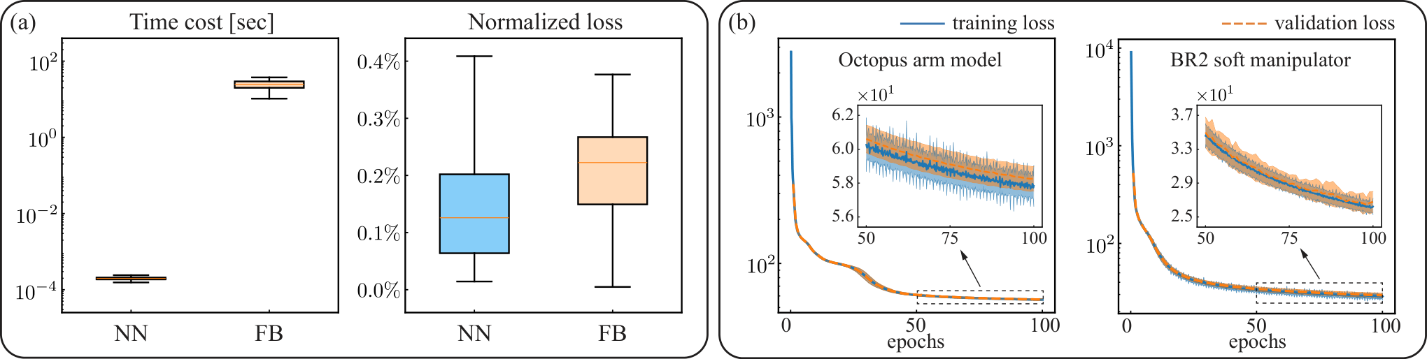
The repeated solve is the computational bottleneck. The neural method reduces reconstruction time by over five orders of magnitude in the reported benchmark, with normalized objective loss on a comparable scale. Training curves summarize fifty independent runs. Figure 3 from the preprint.
Figure 3 compares the learned reconstruction with the previous forward-backward algorithm. Five orders of magnitude corresponds to a factor of 100,000. This comparison measures the reconstruction calculation once marker poses are available; camera acquisition, tracking, communication, and any later control calculation have their own timing costs.
The accuracy comparison uses the reconstruction objective, normalized by the measurement weight and number of markers. It supports the claim that the speed improvement preserves a comparable level of fit under that objective. The separate demonstrations below show what the resulting shapes and strains look like.
Recovering six strain fields in a simulated octopus arm
The first testbed is a 20 cm tapered muscular arm simulated with COOMM and Elastica. Energy-shaping control drives reaching motions toward 27 targets distributed through a three-dimensional workspace. Eight virtual markers provide the observations.
The network receives 72 input values and predicts the 24 coefficients representing all six strain modes. In simulation, the underlying strain fields are available, so we can compare the reconstructed profiles with the simulator's ground truth.
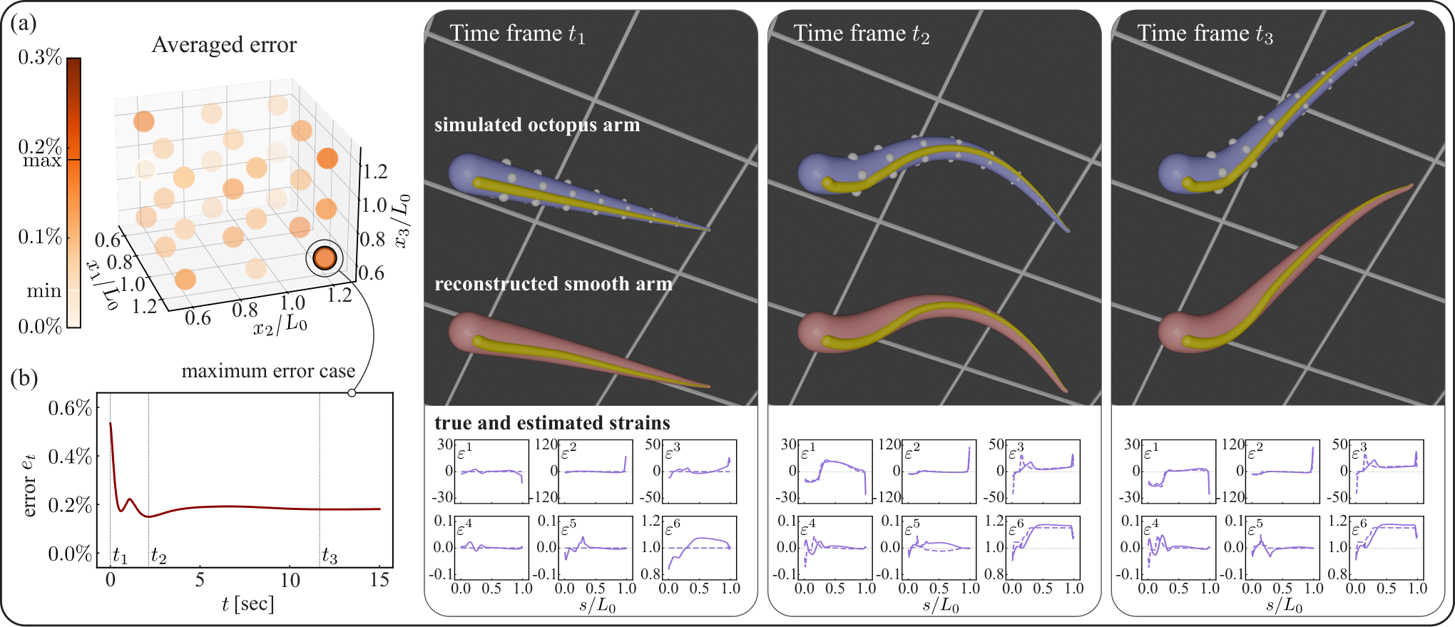
Sparse poses recover a distributed deformation. The snapshots show the reaching trajectory with the largest time-averaged error among the tested targets. Solid strain curves are estimates; dashed curves come from the simulator. Figure 4 from the preprint.
For all 27 reaching trajectories, the time-averaged reconstruction error is below the reported 0.2% level. This percentage has a specific definition: it is the mean marker-pose mismatch, combining squared position differences normalized by arm length squared and squared orientation-matrix differences normalized by eight.
It therefore measures how well the reconstructed poses agree with the observations. It does not translate directly into a position error in millimeters or a percentage error in every strain field. The strain comparisons provide additional, separate evidence about the deformation recovered between markers.
From simulation to a physical pneumatic arm
The second testbed is a 30 cm BR² pneumatic manipulator. Its three pressure inputs produce bending and twisting in either direction. Three ring markers carry reflective tags, and a Vicon motion-capture system supplies their poses at 100 Hz. A complementary filter stabilizes the pose readings before reconstruction.
The training basis comes from COBRA, a simulator for the BR² arm. For this experiment, the model assumes the arm is inextensible and unshearable, so the learned variables are the three angular strains: two bends and twist. Three PCA components per angular strain give nine network outputs from 27 inputs.
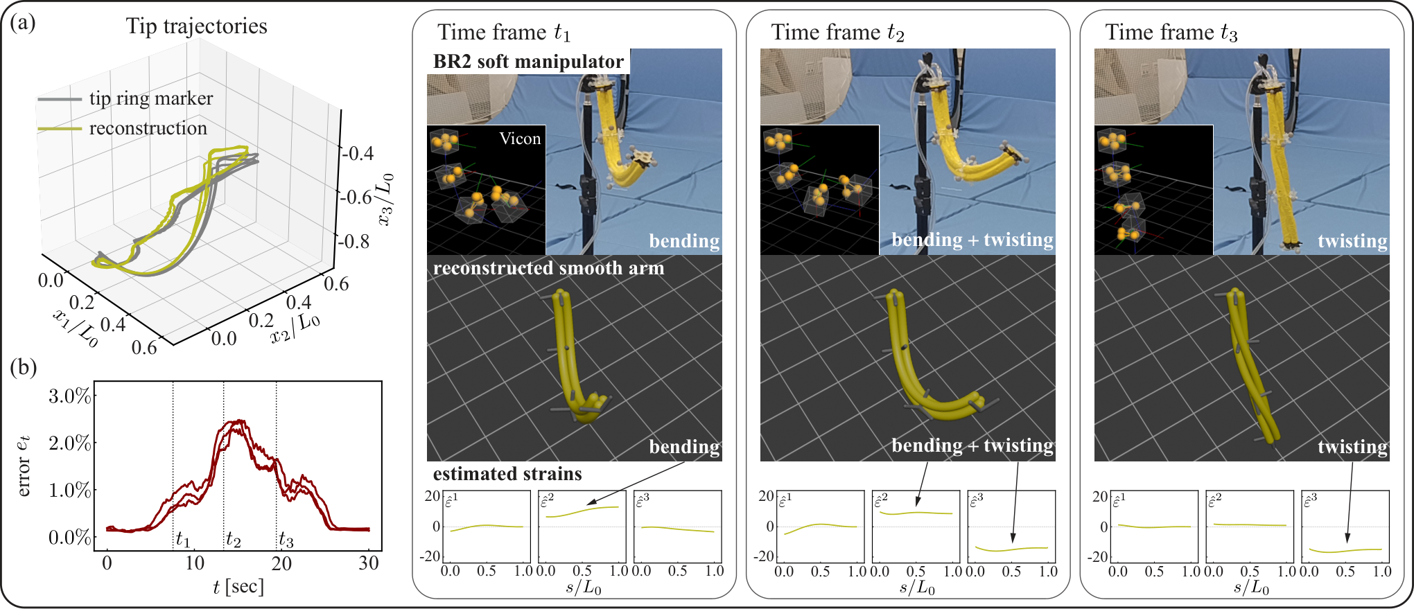
A simulation-trained estimator follows a real arm. The arm bends, adds twist, releases bending, and releases twist over three repeated cycles. The measured tip trajectory and marker frames are compared with the reconstruction. Figure 5 from the preprint.
The experiment reconstructs the arm in real time as it moves through bending, combined bending and twisting, and nearly straight twisting. The repeated trajectories and error curves show consistent behavior across three cycles.
This demonstrates transfer from simulation-generated training data to a physical manipulator. The hardware evaluation compares against measured marker poses and visually checks the reconstructed shape; it does not provide independent measurements of strain everywhere along the physical arm. The six-mode reconstruction is demonstrated in the octopus simulation, while the BR² experiment uses the more restricted model described above.
What “fast and smooth” makes possible
The extension preserves the central aim of the earlier vision-based work: infer continuous deformation from sparse observations while using mechanics to connect the gaps. The learned representation makes that inference fast enough to accompany a live stream of marker measurements.
“Smooth” refers to variation along the arm. The network reconstructs each time frame independently. Its present formulation does not learn temporal dynamics, and the paper leaves dynamic state estimation, more complex motions such as bend propagation, and sensory feedback control as future directions.
The basis, mechanical parameters, marker arrangement, and simulated workspace still shape what can be reconstructed reliably. New deformation patterns or a different robot can require a new basis and training data. Within the evaluated settings, the result is a practical step toward giving soft robots a continuously updated account of their own posture and deformation.
Paper and attribution
This post is based on A Neural Network-Based Framework for Fast and Smooth Posture Reconstruction of a Soft Continuum Arm, by Tixian Wang, Heng-Sheng Chang, Seung Hyun Kim, Jiamiao Guo, Ugur Akcal, Benjamin Walt, Darren Biskup, Udit Halder, Girish Krishnan, Girish Chowdhary, Mattia Gazzola, and Prashant G. Mehta, published in ICRA 2025, pp. 14015–14022. Tixian Wang and Heng-Sheng Chang contributed equally.
The method and results described here follow the published paper. Figures 2–5 are reproduced from the September 19, 2024 arXiv preprint, with explanatory captions supplied here. The figure assets retain the source's CC BY-NC-SA 4.0 license.
The implementation is available on GitHub. For the optimization method that this work extends, see the earlier post, Seeing How Soft Arms Deform: From Camera Images to Six Strain Fields. The BibTeX below cites the published conference paper.
Citation
@inproceedings{wang2025reconstruction,
  title = {A Neural Network-Based Framework for Fast and Smooth Posture Reconstruction of a Soft Continuum Arm},
  author = {Wang, Tixian and Chang, Heng-Sheng and Kim, Seung Hyun and Guo, Jiamiao and Akcal, Ugur and Walt, Benjamin and Biskup, Darren and Halder, Udit and Krishnan, Girish and Chowdhary, Girish and Gazzola, Mattia and Mehta, Prashant G.},
  booktitle = {2025 IEEE International Conference on Robotics and Automation (ICRA)},
  pages = {14015--14022},
  year = {2025},
  doi = {10.1109/ICRA55743.2025.11128142},
  url = {https://doi.org/10.1109/ICRA55743.2025.11128142}
}